Identification of protein-protein interactions between PRC2 to its accessory subunits AEBP2, PHF19, MTF2 and EPOP (NSMB 2019)
Emma Gail
2019-12-03
A Brief Introduction
This tutorial shows how the analysis of BS3 XL-MS data was performed by Zhang et al. 2019 (see References below and here for the source data). This data is mainly files processed by pLink (versions 1 and 2) as well as FASTA files, which crisscrosslinkeR will use for its analysis.
In this tutorial, we will cover:
- data filtration
- sequence alignment to UniProt and PDB files
- data visualization
Install crisscrosslinkeR
If you have not already done so, please install crisscrosslinkeR on your system.
library(devtools)
install_github('egmg726/crisscrosslinker')
It should automatically install all of its dependencies. However, we have also included a list of the packages necessary for this workflow.
Load Libraries
First, we will load all of the libraries that we need for the analysis, including crisscrosslinker1.
library(ggplot2)
library(bio3d)
library(Biostrings)
library(seqinr)
library(RColorBrewer)
library(openxlsx)
library(viridis)
library(crisscrosslinker)
library(stringr)
library(svglite)
library(RCurl)
library(XML)
library(reshape2)
library(curl)
Load Files
To begin the analysis, we will specify the names of the complexes so we can run them each separately.
complexes <- c('PRC2-AEBP2','PRC2-MTF2-EPOP','PRC2-PHF19')
fasta <- seqinr::read.fasta(system.file("extdata/NSMB_FASTA",'PRC2_5m.fasta',
                                        package = 'crisscrosslinker',mustWork = TRUE))
In this case, different names were used for different experiments so we must use a dictionary to be able to match them all2. It is highly recommended to use consistent naming for all of your experiments. If you have the same protein matched to different protein FASTA files that are different sequences across repeats, it is recommended to not use a dictionary and just align them all to a UniProt canonical sequence to match them against each other.
protein_alternative_names_dict <- read.csv(system.file("extdata/NSMB_misc","PRC2_alternative_dict.csv",
                                                       package = 'crisscrosslinker',mustWork = TRUE),
                                                       fileEncoding="UTF-8-BOM")
head(protein_alternative_names_dict)| original_name | alt_name | X |
|---|---|---|
| SUZ12_Q15022 | HMBP_PrS_SUZ12_CD137 | |
| EZH2_Q15910-2 | HMBP_PrS_EZH2(iso2-BsaI)_CD136 | |
| EED_O75530 | HMBP_PrS_EED_CD138 | |
| RBBP4_Q09028 | HMBP_PrS_RBBP4_CD139 | |
| AEBP2_Q6ZN18 | HMBP_PrS_AEBP2_CD140 | |
| PHF19_Q5T6S3 | PHF19 | HMBP_PrS_PHF19 |
In this case, we will start by processing just 1 of the 3 complexes. complexes[1] corresponds to the PRC2-AEBP2 complex3:
sys.dir <- system.file("extdata/NSMB_XLMS",package = 'crisscrosslinker',mustWork = TRUE)
xlms.files <- list.files(path=sys.dir)[startsWith(list.files(path=sys.dir),complexes[1])]
xlms.files
## [1] "PRC2-AEBP2 _4.xlsx" "PRC2-AEBP2_1.xlsx" "PRC2-AEBP2_2.xlsx"
## [4] "PRC2-AEBP2_3.xlsx" "PRC2-AEBP2_5.xlsx" "PRC2-AEBP2_6.csv"
## [7] "PRC2-AEBP2_7.csv"As you can see, there is a mix of .xlsx and .csv files. However, this is not an issue for the ppi.loadData.
From this point on, most of the functions we will use will have the prefix ppi. This stands for protein-protein interaction and is used to distinguish these functions from the protein-RNA interaction functions in crisscrosslinkeR which use the prefix rbd for RNA-binding domain.
#current error with loading csv files
xlms.data <- ppi.loadData(xlms.files,fasta,file_directory = sys.dir)
## Loaded as readline
## Loaded as readlineCombine Data
The original_name must correspond with the name used in the FASTA file. Any name listed in the subsequent columns will be changed to that of the first row.
xlms.df <- ppi.combineData(xlms.data, fasta,
                           protein_alternative_names_dict = protein_alternative_names_dict)
Filtering Data
Since we have 7 repeats, we can check to see how many of these crosslinking events occur more than once.
table(xlms.df$freq)| Var1 | Freq |
|---|---|
| 1 | 134 |
| 2 | 43 |
| 3 | 22 |
| 4 | 7 |
| 5 | 6 |
Var1 represents the number of replicates where a given crosslink has observed, where Freq represents the total number of times such observation occurred across the entire experiment. For instance, while considering all 5 replicates that were included in the experiment used for this example, there were only 6 crosslinking events that were detected across all 5 replicates (bottom row), while 134 of the crosslinking events were identified in only one replicate. Hence, this step can be used to assess the overall reproducibility across replicates, before weeding out irreproducible crosslinking events.
We can also visualize this with a histogram:
qplot(xlms.df$freq,
      ylab = 'Frequency',
      xlab = 'Number of Repeats')
Frequency of XL sites
The vast majority occur in just 1 repeat, so it is important to filter these results so that we can visualize only signficant results. We previously defined significant linked-peptides if they are showing up in at least two replicates or have a p-value of less than 1e-4 (Zhang et al. 2019).
This can be done when processing the data by using the cutoffs within the combineData function or after the fact with conditional statements. For the purposes of this demonstration, we will re-process the data again to show how to filter it.
xlms.df.filt <- ppi.combineData(xlms.data,fasta,protein_alternative_names_dict = protein_alternative_names_dict,freq_cutoff = 2,score_cutoff = 1e-04,cutoff_cond = 'or')Let’s see how the frequencies of our crosslinking sites look now:
table(xlms.df.filt$freq)##
## 1 2 3 4 5
## 75 43 22 7 6As we can see, the frequency of XL sites that only show up 1 time is the highest (75) whereas the rest of the groups (2 to 5) were not changed.
In this case, many of the crosslinking events with freq < 2 are still there since they had significant p-values.
Match to UniProt
In this case, the proteins used in the experiment do not have sequences that match up exactly to the UniProt canonical sequences and have slightly different N-terminals, including few amino acids that remained after tag cleavage. However, this is not an issue as the canonical sequence can be aligned to the experimental sequence using ppi.matchUniprot.
First, a table needs to be made containing the protein names in the FASTA file and their corresponding UniProt IDs.
prc2.alignIDs<- read.csv(system.file("extdata/NSMB_misc",'PRC2_protein_dict.csv',
                                     package = 'crisscrosslinker',
                                     mustWork = TRUE))[,1:2]
colnames(prc2.alignIDs) <- c('ProteinName',"UniProtID")
prc2.alignIDs| ProteinName | UniProtID |
|---|---|
| EZH2_Q15910-2 | Q15910-2 |
| EED_O75530 | O75530 |
| RBBP4_Q09028 | Q09028 |
| SUZ12_Q15022 | Q15022 |
| AEBP2_Q6ZN18 | Q6ZN18-2 |
The ProteinName column should correspond to the names within the FASTA file and the UniProtID should be a valid UniProt ID. If a specific isoform is needed, this should be designated by “id-isoform”. If a specific isoform is not specified, the sequence of the UniProt “canonical isoform” will be imported. If you already have sequences that you would like to use, you can input them in a third column: UniprotSeq. Otherwise they will be retrieved by the UniProt website.
They will then be aligned using the following function:
xlink.df.uniprot <- ppi.matchUniprot(xlms.df.filt,fasta,prc2.alignIDs)
head(xlink.df.uniprot[,c('pro','pro_pos1','pro_pos2')])| pro | pro_pos1 | pro_pos2 | |
|---|---|---|---|
| 1 | EZH2_Q15910-2(43)-EZH2_Q15910-2(34) | 39 | 30 |
| 2 | SUZ12_Q15022(737)-SUZ12_Q15022(741) | 732 | 736 |
| 3 | EZH2_Q15910-2(578)-EZH2_Q15910-2(303) | 574 | 299 |
| 4 | EZH2_Q15910-2(643)-EZH2_Q15910-2(722) | 639 | 718 |
| 6 | RBBP4_Q09028(216)-RBBP4_Q09028(160) | 212 | 156 |
| 7 | SUZ12_Q15022(725)-SUZ12_Q15022(741) | 720 | 736 |
In this table, ‘pro_pos1’ and ‘pro_pos2’ represent the new amino acid numbering assigned to the two amino acids in each pair of cross-linked residues after the alignment to the corresponding UniProt sequence(s). Accordingly, the amino acids numbering are slightly different than within the protein(s) used for the actual experiment (as indicated by pLink output, under ‘pro’) and some have been replaced with NA. In this case, this is because the N-terminal sequence is different from that of the UniProt sequences used due to the vectors used in the experiment.
We are not interested in those positions which have not been matched to a UniProt position so we will omit them from our final analysis.
xlink.df.uniprot <- na.omit(xlink.df.uniprot)Export to xiNET
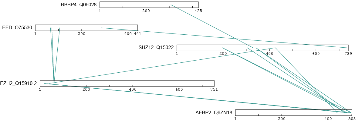
Once the proteins have been aligned to the UniProt sequence of our choosing, we can then visualize them. An easy and popular way to do this is to input them into the web server xiNET4. We can directly translate this data into one that can be understood by their server using the following function:
xlink.xinet <- ppi.xinet(xlink.df.uniprot)
colnames(xlink.xinet)
## [1] "PepPos1" "PepPos2" "PepSeq1" "PepSeq2" "LinkPos1" "LinkPos2" "Protein1"
## [8] "Protein2" "Score"We can then write the file and upload it to their server for use online along with a FASTA file containing the UniProt sequences.
write.csv(xlink.xinet,"PRC2-AEBP2_xinet.csv")If you do not have a FASTA file containing the sequences of the UniProt sequences, you can download them using the download_fasta argument within ppi.matchUniprot or individually by using the uniprot.fasta function for each one individually. This will download them to your working directory so you can upload them to the xiNET server. You will need both in order to visualize them on xiNET.
However, you will have to replace the UniProt name with that of your protein name in order for xiNET to recognize the match if downloading them from online.
You should get an image like this after uploading to xiNET5:
Match to PDB
In this section, we will match our sequences to a known structure using a PDB accession number for 3D visualization.
We will first add to our alignIDs table with the PDB accession number that we want to use.
prc2.alignIDs$PDB <- rep('6C23',nrow(prc2.alignIDs))| ProteinName | UniProtID | PDB |
|---|---|---|
| EZH2_Q15910-2 | Q15910-2 | 6C23 |
| EED_O75530 | O75530 | 6C23 |
| RBBP4_Q09028 | Q09028 | 6C23 |
| SUZ12_Q15022 | Q15022 | 6C23 |
| AEBP2_Q6ZN18 | Q6ZN18-2 | 6C23 |
In this case, we will not identify the chains since one protein on this particular structure can be covered by multiple chains. We can see this with the protein EZH2 (the multiple chains are highlighted with the red box):

Using the functions ppi.alignPDB and ppi.matchPDB3
In order to visualize our sequences, we want to be able to align them to our chosen PDB structure. This can be done using the ppi.alignPDB function with our loaded FASTA file as well as the table we created before.
pdb_numbering <- ppi.alignPDB(fasta_file = fasta,
                              alignIDs=prc2.alignIDs,
                              uniprot2pdb=TRUE)
The uniprot2pdb variable will first align the FASTA sequence to its corresponding canonical sequence in Uniprot to have the most accurate match rather than aligning directly to the PDB sequence (which may be incomplete and lead to mismatches). You can directly align the FASTA sequence to the PDB sequences by setting uniprot2pdb to FALSE, but this is not recommended in most cases.
Once we have a list that matches each of the FASTA sequences to the PDB file, the next step is to actually use this information to adjust the numbering originally found in xlms.df.filt to the PDB file so we can eventually map them on the structure.
xlink.df.filt.pdb <- ppi.matchPDB3(xlms.df.filt,
                                   pdb_numbering = pdb_numbering)
The new data.frame contains the same information as before, with 3 additional columns
colnames(xlink.df.filt.pdb)## [1] "seq" "pro" "freq" "freq_color" "files"
## [6] "pro_pos1" "pro_pos2" "pro_name1" "pro_name2" "pep_seq1"
## [11] "pep_seq2" "pep_pos1" "pep_pos2" "score" "dist"
## [16] "pdb1" "pdb2"We can see the new columns here:
head(xlink.df.filt.pdb[,c('dist','pdb1','pdb2')])| dist | pdb1 | pdb2 | |
|---|---|---|---|
| 1 | 13.810405 | 6C23_C | 6C23_C |
| 2 | NA | - | - |
| 3 | NA | 6C23_K | 6C23_K |
| 4 | 5.748707 | 6C23_K | 6C23_K |
| 6 | 15.024473 | 6C23_N | 6C23_N |
| 7 | NA | - | - |
distrefers to the distance in Angstroms between the two crosslinked amino acids. If one or both of the amino acids are unable to be mapped to the structure,NAwill be produced instead.pdb1is the PDB and chain corresponding to the first crosslinked amino acid (for example, if the amino acid is found on chain C of the 6C23 structure, it will be designated as 6C23_C).pdb2corresponds to the second crosslinked amino acid. It has the same format aspdb1.
We will omit results that have the value NA to retrieve only those which have both amino acids mapped to a chain on the protein structure.
xlink.df.filt.pdb <- na.omit(xlink.df.filt.pdb)
unique(xlink.df.filt.pdb$pdb1)
## [1] "6C23_C" "6C23_K" "6C23_N" "6C23_L" "6C23_A" "6C23_Q" "6C23_M" "6C23_P"You can see that there are matches that expand beyond the chains we have designated. This is due to the fact that the chains on this structure can cover different areas of the same protein sequence.
Using the ppi.distAnalysis function
In order to assess if the distances we see are random, we can use the function ppi.distAnalysis. This function will produce a histogram that compares randomly chosen lysines within the protein complex to those calculated in ppi.matchPDB3.
You can visualize this below:
xlink.df.filt.pdb <- na.omit(xlink.df.filt.pdb)
set.seed(224)
ppi.distAnalysis(xlink.df.filt.pdb)
## Note: Accessing on-line PDB file
## HEADER GENE REGULATION 05-JAN-18 6C23
A comparison of random lysine-lysine interactions (control) with distances derived from experimentally obtained crosslinks.
A comparison between the distribution of distances between pairs of randomly selected lysins (‘Control’) to the distribution of distances measured between experimentally-identified lysin-lysine crosslinked pairs (‘Experimental’). These functions allow you to directly compare randomly distributed distances versus the real distances7. Under good experimental conditions and assuming that the correct structure (PDB) was selected, the distribution of the ‘Experimental’ distances will be determined by the linker length while the distribution of the ‘Control’ distances is determined by the size, shape and distribution of lysines within the structure, as represented in the PDB file used.6
Session Info
devtools::session_info()## ─ Session info ───────────────────────────────────────────────────────────────
## setting value
## version R version 3.6.1 (2019-07-05)
## os macOS Mojave 10.14.3
## system x86_64, darwin15.6.0
## ui X11
## language (EN)
## collate en_US.UTF-8
## ctype en_US.UTF-8
## tz Australia/Melbourne
## date 2019-12-03
##
## ─ Packages ───────────────────────────────────────────────────────────────────
## package * version date lib
## ade4 1.7-13 2018-08-31 [1]
## assertthat 0.2.1 2019-03-21 [1]
## backports 1.1.5 2019-10-02 [1]
## bio3d * 2.3-4 2018-04-03 [1]
## BiocGenerics * 0.30.0 2019-05-02 [1]
## Biostrings * 2.52.0 2019-05-02 [1]
## bitops * 1.0-6 2013-08-17 [1]
## callr 3.3.2 2019-09-22 [1]
## cli 1.1.0 2019-03-19 [1]
## codetools 0.2-16 2018-12-24 [1]
## colorspace 1.4-1 2019-03-18 [1]
## crayon 1.3.4 2017-09-16 [1]
## crisscrosslinker * 0.9 2019-10-22 [1]
## curl * 4.2 2019-09-24 [1]
## desc 1.2.0 2018-05-01 [1]
## devtools 2.2.1 2019-09-24 [1]
## digest 0.6.22 2019-10-21 [1]
## dplyr 0.8.3 2019-07-04 [1]
## ellipsis 0.3.0 2019-09-20 [1]
## evaluate 0.14 2019-05-28 [1]
## fs 1.3.1 2019-05-06 [1]
## gdtools 0.2.1 2019-10-14 [1]
## ggplot2 * 3.2.1 2019-08-10 [1]
## glue 1.3.1 2019-03-12 [1]
## gridExtra 2.3 2017-09-09 [1]
## gtable 0.3.0 2019-03-25 [1]
## highr 0.8 2019-03-20 [1]
## htmltools 0.4.0 2019-10-04 [1]
## httr 1.4.1 2019-08-05 [1]
## IRanges * 2.18.3 2019-09-24 [1]
## jsonlite 1.6 2018-12-07 [1]
## knitr 1.26 2019-11-12 [1]
## labeling 0.3 2014-08-23 [1]
## lattice 0.20-38 2018-11-04 [1]
## lava 1.6.6 2019-08-01 [1]
## lazyeval 0.2.2 2019-03-15 [1]
## magrittr 1.5 2014-11-22 [1]
## MASS 7.3-51.4 2019-03-31 [1]
## Matrix 1.2-17 2019-03-22 [1]
## memoise 1.1.0 2017-04-21 [1]
## munsell 0.5.0 2018-06-12 [1]
## openxlsx * 4.1.3 2019-11-07 [1]
## pillar 1.4.2 2019-06-29 [1]
## pkgbuild 1.0.6 2019-10-09 [1]
## pkgconfig 2.0.3 2019-09-22 [1]
## pkgload 1.0.2 2018-10-29 [1]
## plyr 1.8.4 2016-06-08 [1]
## prettyunits 1.0.2 2015-07-13 [1]
## processx 3.4.1 2019-07-18 [1]
## prodlim 2019.10.13 2019-11-03 [1]
## ps 1.3.0 2018-12-21 [1]
## purrr 0.3.3 2019-10-18 [1]
## R6 2.4.1 2019-11-12 [1]
## RColorBrewer * 1.1-2 2014-12-07 [1]
## Rcpp 1.0.3 2019-11-08 [1]
## RCurl * 1.95-4.12 2019-03-04 [1]
## remotes 2.1.0 2019-06-24 [1]
## reshape2 * 1.4.3 2017-12-11 [1]
## rlang 0.4.1 2019-10-24 [1]
## rmarkdown 1.17 2019-11-13 [1]
## rprojroot 1.3-2 2018-01-03 [1]
## S4Vectors * 0.22.1 2019-09-09 [1]
## scales 1.0.0 2018-08-09 [1]
## seqinr * 3.6-1 2019-09-07 [1]
## sessioninfo 1.1.1 2018-11-05 [1]
## stringi 1.4.3 2019-03-12 [1]
## stringr * 1.4.0 2019-02-10 [1]
## survival 3.1-7 2019-11-09 [1]
## svglite * 1.2.2 2019-05-17 [1]
## systemfonts 0.1.1 2019-07-01 [1]
## testthat 2.3.0 2019-11-05 [1]
## tibble 2.1.3 2019-06-06 [1]
## tidyselect 0.2.5 2018-10-11 [1]
## tufte * 0.5 2019-05-12 [1]
## usethis 1.5.1 2019-07-04 [1]
## viridis * 0.5.1 2018-03-29 [1]
## viridisLite * 0.3.0 2018-02-01 [1]
## withr 2.1.2 2018-03-15 [1]
## xfun 0.11 2019-11-12 [1]
## XML * 3.98-1.20 2019-06-06 [1]
## xml2 1.2.2 2019-08-09 [1]
## XVector * 0.24.0 2019-05-02 [1]
## yaml 2.2.0 2018-07-25 [1]
## zip 2.0.4 2019-09-01 [1]
## zlibbioc 1.30.0 2019-05-02 [1]
## source
## CRAN (R 3.6.0)
## CRAN (R 3.6.0)
## CRAN (R 3.6.0)
## CRAN (R 3.6.0)
## Bioconductor
## Bioconductor
## CRAN (R 3.6.0)
## CRAN (R 3.6.0)
## CRAN (R 3.6.0)
## CRAN (R 3.6.1)
## CRAN (R 3.6.0)
## CRAN (R 3.6.0)
## Github (egmg726/crisscrosslinker@9729555)
## CRAN (R 3.6.0)
## CRAN (R 3.6.0)
## CRAN (R 3.6.0)
## CRAN (R 3.6.1)
## CRAN (R 3.6.0)
## CRAN (R 3.6.0)
## CRAN (R 3.6.0)
## CRAN (R 3.6.0)
## CRAN (R 3.6.0)
## CRAN (R 3.6.0)
## CRAN (R 3.6.0)
## CRAN (R 3.6.0)
## CRAN (R 3.6.0)
## CRAN (R 3.6.0)
## CRAN (R 3.6.0)
## CRAN (R 3.6.0)
## Bioconductor
## CRAN (R 3.6.0)
## CRAN (R 3.6.0)
## CRAN (R 3.6.0)
## CRAN (R 3.6.1)
## CRAN (R 3.6.0)
## CRAN (R 3.6.0)
## CRAN (R 3.6.0)
## CRAN (R 3.6.1)
## CRAN (R 3.6.1)
## CRAN (R 3.6.0)
## CRAN (R 3.6.0)
## CRAN (R 3.6.0)
## CRAN (R 3.6.0)
## CRAN (R 3.6.0)
## CRAN (R 3.6.0)
## CRAN (R 3.6.0)
## CRAN (R 3.6.0)
## CRAN (R 3.6.0)
## CRAN (R 3.6.0)
## CRAN (R 3.6.0)
## CRAN (R 3.6.0)
## CRAN (R 3.6.0)
## CRAN (R 3.6.0)
## CRAN (R 3.6.0)
## CRAN (R 3.6.0)
## CRAN (R 3.6.0)
## CRAN (R 3.6.0)
## CRAN (R 3.6.0)
## CRAN (R 3.6.0)
## CRAN (R 3.6.0)
## CRAN (R 3.6.0)
## Bioconductor
## CRAN (R 3.6.0)
## CRAN (R 3.6.0)
## CRAN (R 3.6.0)
## CRAN (R 3.6.0)
## CRAN (R 3.6.0)
## CRAN (R 3.6.0)
## CRAN (R 3.6.0)
## CRAN (R 3.6.0)
## CRAN (R 3.6.0)
## CRAN (R 3.6.0)
## CRAN (R 3.6.0)
## CRAN (R 3.6.0)
## CRAN (R 3.6.0)
## CRAN (R 3.6.0)
## CRAN (R 3.6.0)
## CRAN (R 3.6.0)
## CRAN (R 3.6.0)
## CRAN (R 3.6.0)
## CRAN (R 3.6.0)
## Bioconductor
## CRAN (R 3.6.0)
## CRAN (R 3.6.0)
## Bioconductor
##
## [1] /Library/Frameworks/R.framework/Versions/3.6/Resources/libraryNotes
The PyMOL aspect of analysis was not done for this particular workflow. An upcoming tutorial will explore this further in detail.
It should be noted that for this particular analysis, domains were built manually by the user. A tutorial on how to do this automatically will be included in the next tutorial.
References
Combe, C. W., Fischer, L. & Rappsilber, J. xiNET: Cross-link Network Maps With Residue Resolution. Molecular & Cellular Proteomics : MCP 14, 1137-1147, doi:10.1074/mcp.O114.042259 (2015).
Yang, B. et al. Identification of cross-linked peptides from complex samples. Nature Methods 9, 904-906, doi:10.1038/nmeth.2099 (2012)
Zhang, Q. et al. RNA exploits an exposed regulatory site to inhibit the enzymatic activity of PRC2. Nature Structural & Molecular Biology, doi:10.1038/s41594-019-0197-y (2019).
crisscrosslinkeRis working to make sure that all dependencies are included to make sure that no errors occur when executing necessary functions.↩Protein names can be spread over multiple columns (as shown in the below table). However, the first column must be the protein name that matches the FASTA file provided.↩
Separating your data by the experimental conditions used and/or biological system is a good first step in order to first identify crosslinks that repeat in multiple replicates. However, you can also do a differential analysis by analyzing all of your data at once.↩
A successor of xiNET has recently gone live: xiVIEW. xiVIEW has more viewing options, but the xiNET output from
crisscrosslinkeRcan also be read by xiVIEW. For more information on xiNET upload requirements please see here.↩You can also include domains as part of the image output. A function to automatically do this and generate a compatible table for xiNET will be released soon. However, xiNET’s successor (xiVIEW) contains the functionality.↩
Currently, this functionality only works for lysine-lysine interactions.↩